
What the Nyquist Theorem Actually Says (and What It Doesn't)
The Nyquist-Shannon sampling theorem is the mathematical foundation for converting any continuous analog signal into a digital one. It tells us the minimum sample rate required to capture all the information in a signal without losing anything to aliasing. IEEE Xplore ieeexplore.ieee.org/document/1697831 reports that the formal theorem comes from Claude Shannon's 1949 paper, building on earlier work by Harry Nyquist in 1928.
The core statement is precise. "if a function contains no frequencies higher than w cycles per second, it's completely determined by giving its ordinates at a series of points spaced 1/(2w) seconds apart." This gives us the famous 2w rule: your sample rate must exceed twice the highest frequency present in your signal.
What the theorem doesn't say is where most engineers get tripped up. It presumes your signal is perfectly band-limited, meaning it contains absolutely zero energy above that w frequency. No real world signal from a camera sensor or a microphone actually meets this ideal. The theorem provides a condition for perfect mathematical reconstruction, not a practical design shortcut for any arbitrary signal. If I'm being honest, I've seen this idealization lead to more under-sampled security camera deployments than I can count.
The theorem also doesn't specify what happens when your signal isn't perfectly band-limited. All the same, it assumes you've already dealt with that, usually with an analog low-pass filter before the ADC. Without that filtering, frequencies above w don't just vanish. They fold back into your sampled data as lower-frequency aliases, corrupting your signal. This gap between the theorem's ideal condition and real world signal behavior is where the practical problems begin. That gap isn't theoretical. It shows up every time you skip the anti-aliasing filter because you think your source is clean enough.
Understanding this ideal versus real distinction is key to diagnosing why your crisp 4K stream sometimes shows strange, wavy artifacts on fine patterns. That's the aliasing we need to tackle next.
How the Signal Chain Breaks: Aliasing, Anti-Aliasing Filters, and Real Headroom

Tackling that aliasing starts with the Nyquist theorem. NIH/NIDCD "Noise-Induced Hearing Loss" reference data shows human hearing spans roughly 20 Hz to 20 kHz. Nyquist dictates you must sample at least twice that highest frequency. A 44.1 kHz CD rate provides a little headroom above 20 kHz for the rolloff of a real anti-aliasing filter. This math isn't an approximation. It's a hard boundary.
One quick disambiguation before we go further: in this article, DSP means digital signal processor, the chip, or digital signal processing, the discipline. It has nothing to do with the ad-tech "demand-side platform" that shares the acronym. Those processors are where the filtered signal ends up. Aliasing can't be corrected after digitization. Once a high frequency folds back into your data, it's indistinguishable from a real signal. That's why the anti-aliasing filter must be analog, placed before the ADC. Every decent ADC front-end has one.
So what does a DSP in practice do? Data from Texas Instruments TMS320 Family Overview indicates it's a microprocessor built for the single-cycle multiply-accumulate math common to signal filters. That's the core engine chewing on the clean, anti-aliased data. But here's the thing, the real magic of current converters is oversampling, which moves the Nyquist limit way up and lets you use a much gentler analog filter. You then digitally downsample to your final rate.
This all connects to the debate over bit depth and headroom. Per Bob Katz, the ear can't distinguish a properly dithered 16-bit recording from 24-bit under normal listening conditions. High-res audio is about the headroom during mixing, not the final playback. That headroom is your margin for error before you clip. It's extra space in the digital domain.
We'll see how these sampling rates play out in the wild next.
Nyquist Rates in Deployed Systems: Telephony, Audio, and Medical Imaging
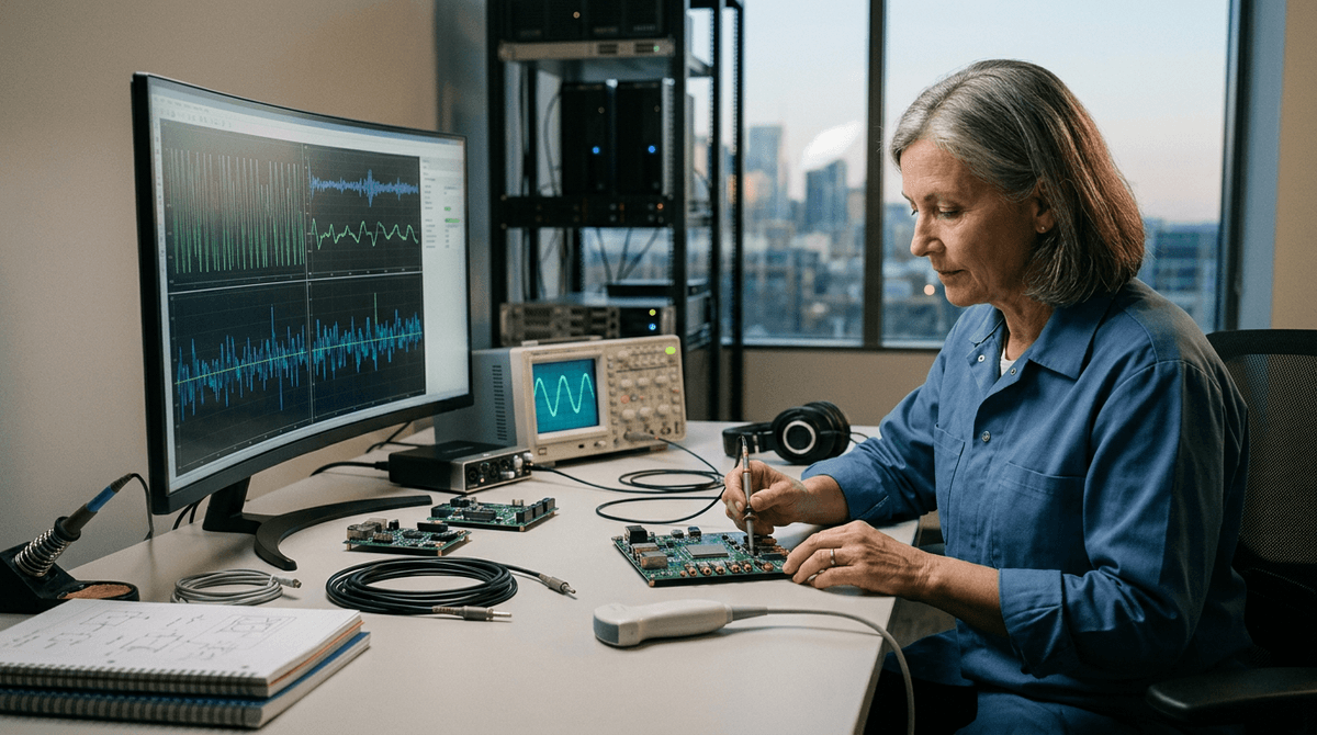
So where do these theoretical limits actually land in production gear? In professional audio and broadcast video, the answer is almost always 48,000 Hz. Data from AES5-2008 r2019 professional audio recommended practice indicates 48 kHz is the standard because it divides evenly into common video frame rates like 24 and 25 fps. 30 fps works cleanly too. This clean divisibility prevents timing errors and simplifies synchronization across big systems, which is why it dominates everything from studio recorders to broadcast consoles.
The classic CD standard tells a different, more historical story. The 44.1 kHz sampling rate was chosen to fit digital audio onto standard PAL video tape used as a storage medium. That's a legacy constraint we've carried for decades. It's a fine rate for final playback, but it doesn't divide cleanly into current video rates, making it a headache for synchronized production workflows.
If you're evaluating high-resolution audio specs, the numbers can look impressive on paper. AES White Paper "High-Resolution Audio" reports that 96 kHz/24-bit audio provides a theoretical dynamic range of 144 dB, compared to 96 dB for 16-bit CD. In reality, most commercial recordings operate far below that ceiling. A quiet vinyl pressing might deliver 60 dB, and a well-treated live room is around 85 dB. The headroom is real for processing, but the finished product rarely demands it.
The core of deployed Nyquist is pragmatic: choose the rate that matches your system's clocking and delivery requirements. The theoretical ceiling matters less than synchronization reliability across your gear. That practical reality leads directly to a deeper issue with how we name these rates.
What the Spec Sheet Doesn't Tell You: Nyquist's Naming Problem and the Kotelnikov Gap
That naming issue is more than academic. It's a gap between the theorem's history and its application, and it hides in the term "Nyquist rate" we just talked about. Most engineers learn it as the Nyquist-Shannon theorem, but the foundational proof actually came first from Vladimir Kotelnikov in 1933. Per the COMSOL blog, his rigorous work was published in the Soviet Union and then lost to the wider world for over a decade. Harry Nyquist's relevant 1928 paper wasn't explicitly about analog signal reconstruction. Shannon then formally unified and popularized the concept in 1949.
This matters because the name on the theorem influences our mental model. We call it the Nyquist rate, but we're often applying Shannon's interpretation of Kotelnikov's proof. The practical reality is that the theorem's requirement, a perfectly band-limited signal, is, as Westcott Design notes, an ideal that no real world signal meets. I've never torn down a camera or an ADC that came with a warning label explaining this. The Kotelnikov gap and the non-ideal behavior it creates go undocumented every time.
So when a spec sheet simply states a "Nyquist-compliant" sampling rate, it's hiding a layer of engineering judgment about anti-aliasing filters and signal assumptions. It's telling you the ideal math, not the field compromise. This historical and technical context is critical before we look at modern techniques that try to sidestep these limits entirely.
Sub-Nyquist Sampling: Compressed Sensing, Sparse Signals, and Where the Floor Actually Moves

The classic Nyquist theorem says you sample at twice the highest frequency of interest to avoid aliasing. That's a sound, conservative floor. Compressed sensing challenges that floor. It argues that if a signal is sparse, meaning most of its possible frequency components are zero, you can reconstruct it perfectly from far fewer samples. The reconstruction isn't a simple formula, though. It's a computationally intensive optimization problem.
The telephone system is a classic, if analog, example of working with sparse signals. ITU-T G.711 found that voice is sampled at 8,000 Hz to capture bandwidth up to 4 kHz. But human speech doesn't use that full 4 kHz spectrum evenly. Energy clusters in narrow bands. The system was engineered around that sparsity long before the math was formalized. If you know your signal's potent bandwidth is much lower than its raw bandwidth, sub-Nyquist techniques become worth evaluating.
Where the floor moves depends entirely on your assumptions. If frequency locations are unknown, Mishali and Eldar's work shows you might pay a factor of two penalty over the ideal sub-Nyquist rate. Stability and reconstruction guarantees become probabilistic rather than absolute. This isn't theory for its own sake. It directly impacts the front-end analog design, the ADC selection, and the processor you'll need to solve the reconstruction equations. Most commercial security gear doesn't touch this because the R&D cost isn't justified for the marginal gain. The exception is in specialized spectral monitoring or scientific imaging where the data's inherent sparsity makes the compute trade-off worthwhile.
The next logical step is pairing these sampling concepts with concrete ADC specs and oversampling rules that hold up in real world noise.
Applying the Nyquist Theorem: ADC Selection, Oversampling Ratios, and Practical Headroom Rules
Taking the Nyquist theorem from a textbook rule to a working ADC selection criterion means looking past the minimum sampling rate. You need to consider the noise floor of your specific signal path and the practical oversampling ratios that give you usable resolution gains. AVR121 reports that oversampling and decimation require some inherent noise in the signal, at least 1 LSB, to toggle the least significant bits effectively. Without that variation, you just get repeated samples. That's no resolution benefit at all.
The relationship between oversampling factor and extra bits follows a predictable pattern, but it's not magic. As the ADC Oversampling Calculator and AN118 outline, each further bit of resolution requires sampling four times faster than the Nyquist rate for your signal of interest. This is a stiff tradeoff against your ADC's maximum throughput and the processing time you can afford.
A lot of the headroom rules floating around are just experience baked into a number, not a core law. Treat a vendor's "effective number of bits" claim as a starting point for your own measurement, not a guarantee. The noise floor of your actual board, with your actual layout and power supply, decides what you really get.
We'll tackle the most prevalent questions on these tradeoffs next.
Frequently Asked Questions
Why is CD audio exactly 44,100 Hz? Because early digital audio was mastered onto PAL video tape, and 294 lines times 50 fields times 3 samples per line works out to 44,100. It also happens to sit just above twice the 20 kHz limit of human hearing, leaving margin for the anti-aliasing filter's rolloff. The number is a storage-format accident that became a permanent standard.
What actually happens if I sample below the Nyquist rate? Frequencies above half your sample rate fold back into your data as lower-frequency aliases. A 30 kHz tone sampled at 44.1 kHz shows up as a phantom 14.1 kHz tone, indistinguishable from a real one. No amount of post-processing can separate them. That's why the anti-aliasing filter has to sit in the analog domain, before the converter.
Why does professional gear use 48 kHz instead of 44.1 kHz? Divisibility. 48,000 divides evenly into 24, 25, and 30 fps video frame rates, which keeps audio and video sample clocks locked without drift. Per AES5, that synchronization convenience matters more in production than the marginal bandwidth difference.
Does oversampling really buy me extra resolution? Yes, with conditions. Per Atmel's AVR121 application note, each extra bit of effective resolution costs a 4x increase in sample rate, and the technique only works if the signal carries at least 1 LSB of natural noise to dither the quantizer. Oversample a perfectly clean DC signal and you just collect identical samples.
Is the theorem named after the wrong person? Arguably. Kotelnikov published the rigorous proof in 1933, before Shannon's 1949 formalization, and Nyquist's 1928 paper wasn't about reconstruction at all. "Nyquist-Shannon" stuck in the English-language literature, and the name matters less than remembering what the theorem assumes: a perfectly band-limited signal that your hardware never actually gives you.