What the FFT Actually Does (and Why the DFT Alone Was Unusable)
Danielson and Lanczos manually computed a size 64 DFT in 140 minutes back in 1942. Cooley and Tukey's 1965 FFT ran a size 2048 complex DFT in 0.02 minutes on an IBM 7094. That's a 32 times larger problem. Finished 7000 times faster. The leap came from swapping O(N squared) work for O(N log N).
O(N²) vs O(N log N): The Arithmetic That Changed Everything
DFT demands every output bin touches every input sample. For N equals 1024 you burn roughly one million operations. Scale to N equals 4096 and it explodes past 16 million. That's a lot of pain. FFT cuts it dramatically. Gilbert Strang called it the most important numerical algorithm of our lifetime.
We don't have easy benchmarks on every embedded MCU today. Still the gap remains brutal on anything without hardware acceleration. One parenthetical aside. Gauss figured out something similar in 1805 but nobody noticed until later. The math always mattered. Execution time is what unlocked real systems.
Dave's Take
Dave's Take: Josh leans hard on the 1965 IBM 7094 numbers. Fair enough for the era. But what's the measured cycle count on a 2026 Cortex M7 at 480 MHz versus the datasheet flop count? Those old mainframe figures don't map cleanly to cache stalls or memory bandwidth. Source on the exact 0.02 minutes?
From Danielson-Lanczos to Cooley-Tukey: 140 Minutes to 0.02 Minutes
Look at the hand calculation. Sixty four points took two hours plus. The IBM 7094 chewed through 2048 points in barely over a second. Cooley Tukey delivered the practical breakthrough. It didn't just make daily DFT work possible, it made it something engineers could actually rely on instead of treating it as a research curiosity.
And yeah the algorithm variants kept improving. Split radix held the record with 4N log base 2 of N minus 6N plus 8 real operations for 35 years. Johnson and Frigo's 2007 tweak shaved about 6 percent more off that. If I'm being honest, these operation counts still feel academic until you profile them on the exact board you are deploying.
The numbers changed how engineers approached signal analysis entirely. A failure mode that shows up later starts here. When your FFT size or radix choice does not match the hardware realities you pay in power or dropped frames. Pick the wrong one and the system never ships on time.
The Cold War Origin Story and the 2025 IEEE Milestone
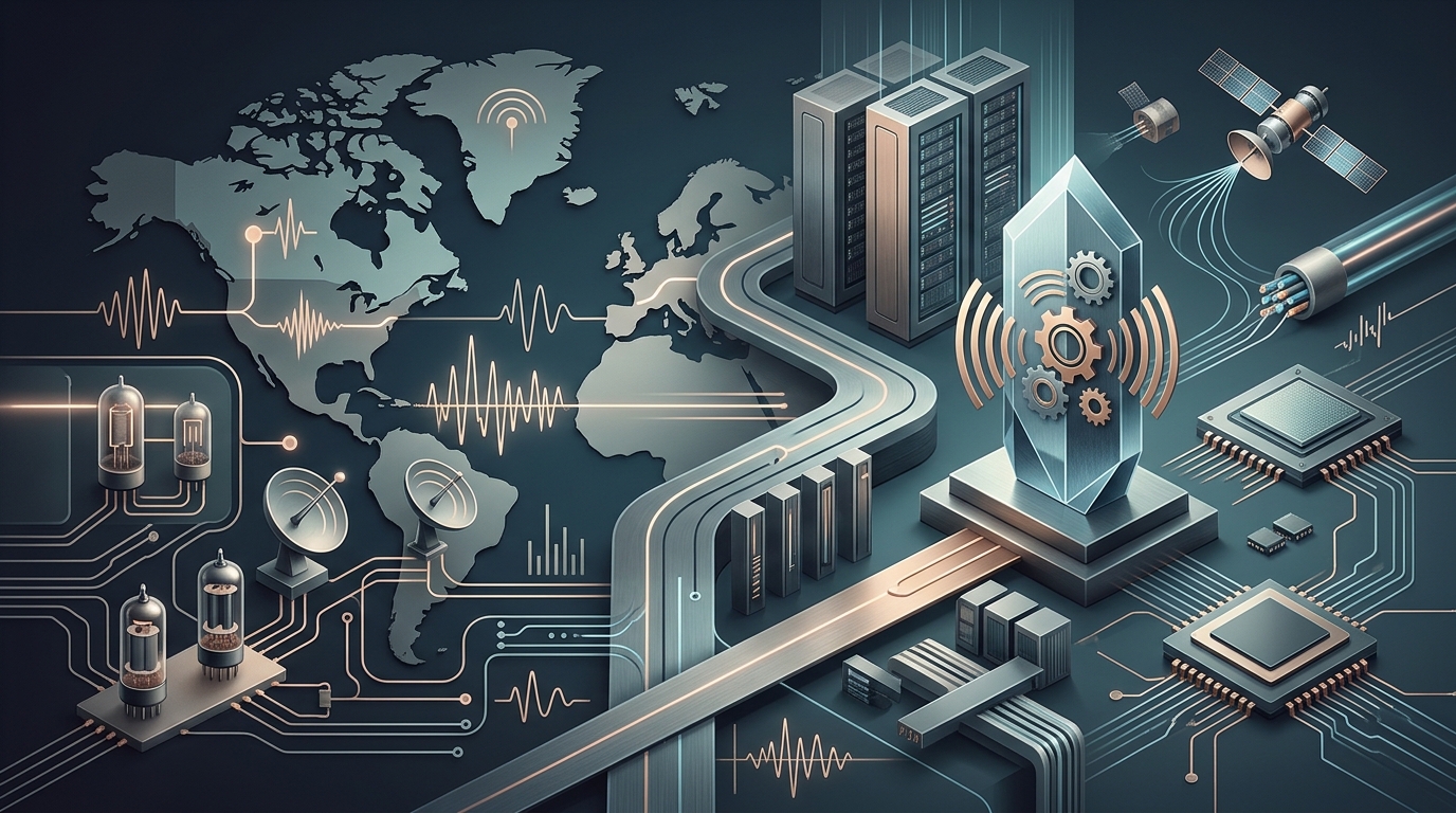
Imagine seismometer traces from suspected Soviet underground tests. That was the classified problem John Tukey needed to solve fast. He developed the core idea for detecting nuclear blasts without waiting weeks for manual Fourier work. Garwin connected Tukey with IBM's James Cooley. He deliberately hid the true purpose from Cooley, a calculated move that kept the military application buried inside what looked like a routine computational project.
John Tukey's Nuclear Test Detection Problem
Tukey conceived the method specifically for that nuclear verification task. Analog methods could not keep up. The Cooley Tukey approach replaced them and made everyday DFT feasible according to Tom Coughlin the 2024 IEEE President in the October 2025 IEEE Spectrum.
Per the same piece, the acceleration turned an impractical calculation into something you could actually use. That's the thing, it worked. We see echoes of that today in sensor hubs running continuous vibration analysis, where the math that once required dedicated hardware now runs on a chip that costs less than a cup of coffee. The origin story explains why the algorithm got so much early attention and funding.
Dave's Take
Dave's Take: The nuclear test story sounds dramatic. But how much of the speedup came from the algorithm versus the IBM 7094's raw horsepower? Compared to what a modern MCU achieves on the same 2048 point task? Garwin's 2024 interview is great color. Still I want the cycle accurate numbers not the legend.
The IBM Watson Plaque and Richard Garwin's Legacy
In June 2025 IEEE awarded IBM Research a Milestone plaque for the first demonstration of the fast Fourier transform in 1964. They installed it at the Watson Research Center office where Cooley worked. Garwin who made the introduction died in 2025. He said in a 2024 IEEE Spectrum interview that linking Cooley and Tukey was the achievement he was most proud of.
The plaque marks more than nostalgia. It recognizes the moment a classified need became foundational infrastructure for everything from audio to 5G. Richard Garwin's role stayed quiet for decades. Now it sits in bronze at the lab.
FFT size and radix choices still bite implementers decades later. They don't change. The Cold War roots don't change the silicon constraints we fight today, and that gap between historical origin and modern consequence is something implementers keep rediscovering every time a new chip family lands.
FFT Size, Radix, and Algorithm Variants: What the Spec Sheet Doesn't Tell You
Power of two constraints dominate most datasheets. 5G NR pushes a maximum FFT size of 4096 points double LTE's 2048 with 3300 active data subcarriers and up to 400 MHz bandwidth. Subcarrier spacing options run 15 30 60 or 120 kHz per 3GPP Release 15 TS 38.211.
Power-of-Two Constraints and Why 4096 Points Matters for 5G NR
You cannot just pick any length. Hardware and libraries assume powers of two for clean butterfly stages. 4096 points lets the modem handle that wide channel without padding tricks that waste spectrum. The jump from 2048 matters when bandwidth doubles.
I notice most vendor spec sheets list the max size but skip the memory traffic it creates on a shared bus. That omission shows up when you stack it with other real time tasks.
Split-Radix vs Cooley-Tukey vs Sparse FFT: When Each One Wins
Split radix held the lowest operation count for 35 years at 4N log base 2 of N minus 6N plus 8 real arithmetic operations. Johnson and Frigo's 2007 modified version cut roughly 6 percent more requiring about 34 over 9 times N log base 2 of N flops per IEEE Transactions on Signal Processing 2007. Cooley Tukey remains the workhorse for general use.
Sparse FFT from MIT in 2012 hits sub linear O of k log N for sparse signals like MRI where most bins sit near zero. It can run 10 times faster but only crosses over versus standard FFT once N reaches 25 000 in one dimension. Adoption stays slow. The lower bound problem on arithmetic complexity remains unsolved. We lack confirmed data on how often real vibration sensors hit that sparsity sweet spot.
Dave's Take
Dave's Take: Johnson and Frigo 2007 looks solid on paper. Is the 6 percent measured on a modern out of order CPU with SIMD or just flop counts? Sparse FFT sounds perfect until you measure setup overhead on a microcontroller. The crossover at N greater than or equal to 25 000 feels theoretical. What's the actual break even on the parts we deploy?
Cache Locality Beats Arithmetic Count on Modern CPUs
Here is the catch. Minimizing arithmetic operations does not always minimize runtime anymore. Cache misses and pipeline bubbles dominate on current chips. FFTW's planner that tunes at runtime often beats hand optimized theoretical winners because it respects memory hierarchy.
Radix choices affect vectorization and locality differently across ARM Cortex parts versus x86. The spec sheet rarely tells you which variant wins on your exact board. Test it. The variant that looks best on paper can lose by 30 percent or more once caches and memory controllers get involved. Pick based on measured latency not just operation tallies. That choice determines whether your 4096 point run finishes in time for the next sample batch or forces dropped data.
Common Failure Modes in the Field

A 512 point FFT on the ESP32 S3 vector unit clocks in at roughly 50 microseconds. That is fast enough for most audio work. The same size on an STM32F4 with CMSIS DSP lands around 120 microseconds. A TI C6748 DSP drops it to 5 microseconds while a Xilinx Zynq FPGA finishes under 1 microsecond. Cost tells its own story. The ESP32 sits at three dollars. The TI part runs fifteen dollars. FPGAs start north of forty dollars.
ESP32-S3 vs STM32F4 vs TI C6748 vs FPGA: 512-Point FFT Timing
Look at the numbers again. ESP32 S3 wins on price and gets the job done for many smart home tasks. Its vector instruction unit handles the heavy lifting without external chips. STM32F4 needs more cycles because CMSIS DSP still runs on a general purpose core. We have covered DSP extensions on ESP32 since the chip launched. The gap widens when sample rates climb. Audio processing runs at 16 to 48 kilohertz. That leaves the DSP 20 to 60 microseconds per sample before the next one arrives. Miss that window and you drop frames.
The TI C6748 and Zynq parts shine in dedicated signal chains. They chew through transforms with headroom to spare. But you pay for it. Three dollars buys an ESP32 that talks nicely to Wi Fi and handles the rest of the IoT stack. Forty dollars for an FPGA changes the BOM fast. Pick based on your latency budget and power envelope.
Dave's Take: These timing numbers look clean. Are they measured on the exact same 512 point real valued input or padded and optimized per vendor? FPGA under 1 microsecond sounds great until you add data movement cost. What is the total system latency once you count DMA setup and memory copies? The spreadsheet rarely matches the scope.
ASIC vs FPGA Energy Per Transform: The 51% Gap That Matters for SKA
An FFT implemented as an ASIC on a 65 nanometer process consumed 0.41 microjoules per transform. The equivalent FPGA burned 0.84 microjoules. That 51 percent energy reduction matters when you scale to thousands of nodes. Radio telescope arrays like SKA run continuous transforms around the clock. Every microjoule saved drops your cooling bill and your solar array size.
Smart home devices usually dodge this math. They use dedicated accelerators inside the SoC or lean on ARM Cortex M cores with DSP extensions. The power difference still shows up in battery powered sensors. The ASIC route looks attractive on paper until you factor in NRE costs and volume requirements. Most of us never hit the numbers that justify a mask set. Stick with the FPGA or MCU until your deployment count justifies the custom silicon. The 0.41 microjoule figure is worth remembering when power budgets tighten.
Common Failure Modes in the Field
One Amazon Echo Dot fifth generation sits on my test bench with seven MEMS microphones feeding a 48 kilohertz 16 bit ADC array. The beamforming and acoustic echo cancellation code runs adaptive filters that update roughly one thousand times per second. It works until the room changes fast. Then the filters chase their own tail and the wake word detector gets confused.
Voice Assistants: Beamforming, AEC, and the Wake-Word Pipeline
The audio chain inside these speakers relies on FFT based beamforming across those seven microphones. Wake word detection runs a tiny 200 to 500 kilobyte model at one to two milliwatts. The local detector fires an interrupt. Everything after that heads to the cloud. According to the Federal Trade Commission staff report nearly 89 percent of manufacturer web pages for these IoT products failed to disclose how long the products would receive software updates. That leaves you wondering how long the FFT routines will stay patched.
The NIST Hardware Roots of Trust project puts it plainly. Because roots of trust are inherently trusted, they must be secure by design. That's not optional. Smart home signal chains we've covered on eg3.com show the same pattern, and the vulnerabilities compound quickly when foundational assumptions go unchecked. The FFT block is only as reliable as the code around it.
Dave's Take: Seven mics at 48 kHz sounds impressive. Compared to what though? Is the AEC update rate measured or just the marketing target? Wake word models under 2 mW are great on the eval board. Real room noise and temperature swings change those numbers. Source on the 89 percent disclosure failure would help too.
5G Modems, OFDM, and the 4096-Point Transform in Your Phone
5G NR needs a 4096 point IFFT at the receiver for OFDM demodulation. The global FFT analyzers market sat at about 300 million dollars in 2024. Projections put it at 600 million by 2033 with an 8.5 percent CAGR. 5G deployment and predictive maintenance drive most of that growth. Your phone handles the heavy transform in dedicated baseband silicon because a general purpose core could never keep up. The latency budget stays tight. Miss it and you lose packets.
Matter 1.5 released in November 2025 added camera and video doorbell types. That bumps demand for MCUs with strong image pipelines. The STM32H7 Chrom ART accelerator pulls ahead here, it's doing the heavy lifting once you're outside the audio band. These transforms scale fast.
Common Failure Modes in the Field
What happens when your library choice adds 50 percent more latency than the datasheet promised? That's not a hypothetical. It happened, and the gap between spec and reality doesn't close itself.
FFTW, CMSIS-DSP, cuFFT, and MKL: Which Library for Which Platform
On modern CPUs minimizing arithmetic count does not minimize execution time. Cache locality, SIMD vectorization width and pipeline utilization dominate. FFTW auto tuning planner often beats theoretically optimal split radix implementations. Intel MKL can run 50 percent faster than FFTW despite using the same algorithmic family. NVIDIA cuFFT version 13.2 updated in April 2026 now supports multi node distributed 3D FFTs through the cuFFTMp API. It scales across up to 16 GPUs tied to one CPU.
CMSIS DSP stays the safe choice for STM32 parts. It knows the Cortex M SIMD intrinsics. The RP2350 with its dual Cortex M33 at 150 megahertz and DSP extensions competes hard at under one dollar. We see the same story on RP2040 versus STM32H7. One has PIO for custom interfaces. The other has deterministic flash and faster ADCs.
Dave's Take: MKL 50 percent faster sounds definitive. Measured on which CPU with which compiler flags? CuFFT across 16 GPUs is impressive for exascale work but what is the actual node to node bandwidth penalty? The arXiv adversarial lower bounds paper from April 2026 raises good questions about sparse FFT validation costs. Does any of this match your bench time?
Failure Modes: Spectral Leakage, Picket Fence Effect, and Wrong N
Spectral leakage appears when the signal does not contain an integer number of cycles inside the capture window. Energy smears across bins. Window functions fix most of it. Hann works for starters. Blackman gives tighter sidelobes at the expense of a wider main lobe. The picket fence effect comes from bin spacing that misses your exact frequency. Wrong N is simpler. Pick a size that is not a power of two and you force Bluestein which runs three to five times slower. An April 2026 arXiv paper set new adversarial lower bounds of Omega k squared for CRT based sparse FFT algorithms. Poor moduli choices make validation cost exceed a dense transform. Test your N. Measure the actual latency.
The RP2350 launched in August 2024 with FPU and DSP extensions that close the gap versus older STM32 parts. Its interpolator peripherals handle sensor curves at zero CPU cost. That matters for vibration work where FFT feeds directly into EKF loops.