What an IIR Filter Actually Does (and Why the Feedback Loop Is the Whole Point)
An IIR filter is a recursive system. The output at any sample depends not only on current and past inputs but also on previous output values. That feedback loop is the defining characteristic. Data from Richard G. Lyons' Understanding Digital Signal Processing indicates this architecture is why IIR filters can achieve a steeper rolloff with fewer coefficients than an equivalent FIR. The trade-off is stability. The feedback coefficients place poles in the filter's transfer function. If those poles drift outside the unit circle due to coefficient quantization or design error, the filter can oscillate or diverge.
An FIR filter has no feedback. All its poles are at the origin. Lyons notes this makes FIRs unconditionally stable. All the same, the cost is latency. A linear-phase FIR introduces a group delay equal to (N-1)/2 samples. AES Convention Paper 10487, "On latency and group delay in DSP audio", quantifies this: a 128-tap FIR at 48 kHz creates about 1.3 ms of delay. That's audible in live monitoring. For latency-sensitive audio work or real-time control loops, that group delay can be a dealbreaker.
If I'm being honest, I've avoided speccing linear-phase FIR filters for live audio monitoring in venue installs for exactly that reason. The latency is measurable and performers notice. IIR filters, with their much lower inherent delay, are often the practical choice despite their stability demands. This efficiency versus stability trade-off is the core engineering decision.
The feedback path is what gives the IIR its power and its peril. Getting the coefficients right is everything. We'll look at the classic design methods for doing that next.
IIR Filter Design Methods: Butterworth, Chebyshev, and Elliptic Compared
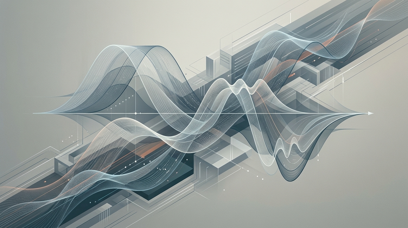
The classic analog filter prototypes give us our starting points. Each makes a separate trade-off between passband fidelity, stopband rejection, and transition sharpness. The Butterworth is your maximally flat option. It's monotonic with a smooth rolloff, making it the go-to when you want no ripple anywhere, at the cost of needing a higher order for a sharp cutoff. The Chebyshev designs split the difference: Type I allows equiripple in the passband for a monotonic stopband, while the inverse Type II keeps the passband flat and puts the ripple in the stopband. Both give you a sharper cutoff than Butterworth at the same order. You're trading ripple for speed.
Then there's the elliptic, or Cauer, filter. It's equiripple in both bands, which mathematically gives you the sharpest possible transition. Per the theory, it meets a given spec with the lowest filter order. Elliptic is often the brute-force choice when you need insane rolloff and can live with the phase distortion.
Your filter choice dictates the computational load and phase response of the entire signal chain. We'll look at how that in practice runs on real hardware next.
How the IIR Signal Chain Runs on Real Hardware
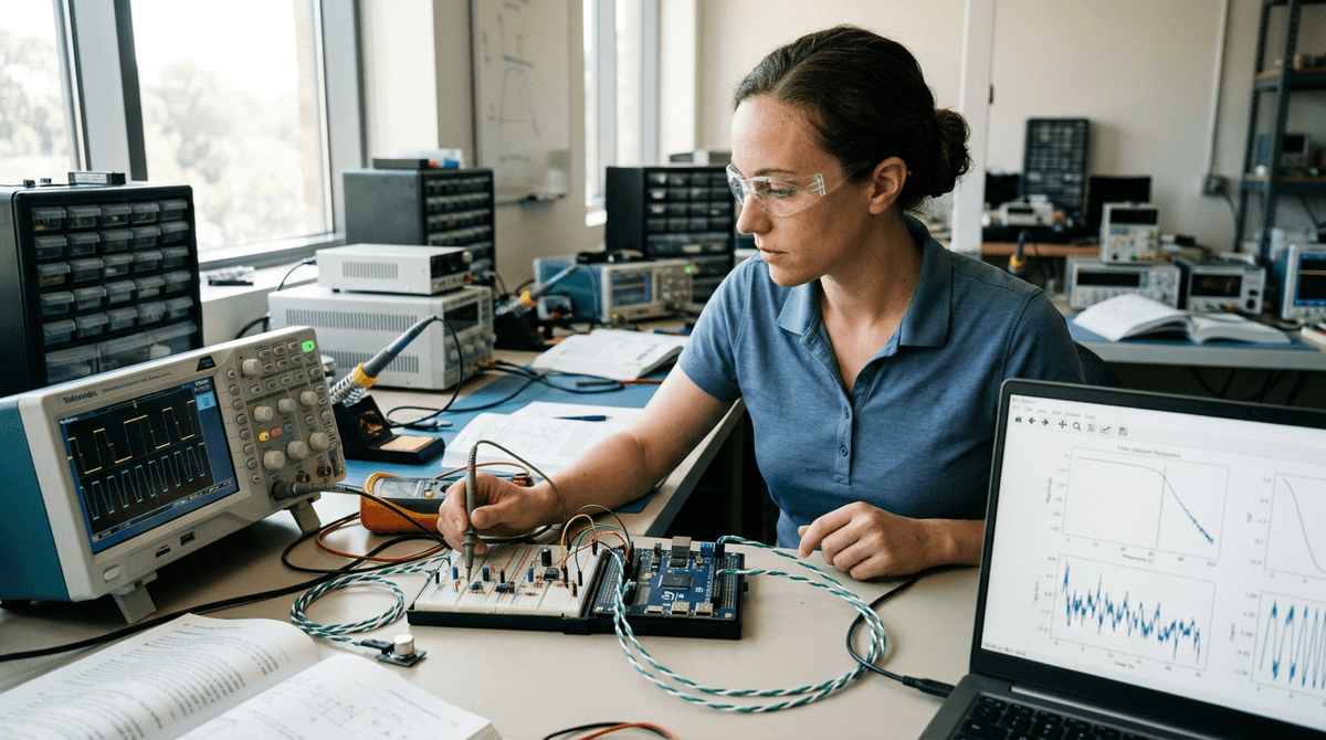
That offloading happens on dedicated silicon. Today's processors designed for signal work, like the ADSP-2156x or Renesas RA6T2, integrate hardware accelerators specifically for IIR filtering. Analog Devices data shows these accelerators consist of their own multiply-accumulate units and local memory, operating somewhat independently from the main core.
The core's job becomes setup and data routing. It initializes a chain of DMA transfers that feed sample data into the accelerator's buffer, writes the start address of this control chain to a pointer register, then kicks off processing. An interrupt signals completion, telling the core the filtered output's ready for the next stage. You can see how this hands off approach saves make-or-break CPU cycles in real-time audio or sensor processing. That's the whole point: once it's running, the core doesn't touch it.
The theoretical "fully offload everything" model rarely plays out in simple embedded designs. As the Renesas documentation notes, the core often has to wait for results to proceed with dependent tasks, which limits parallel gains. That's the catch. The practical choice is between direct replacement or splitting channels between core and accelerator. Pipelining frames is the third option. The right pick depends on your channel count and latency tolerance, plus what else the CPU needs to do.
This is where stability becomes a concern. A direct-form IIR implementation with high-order sections can suffer from coefficient sensitivity and limit cycles. Using a cascade of second-order sections, a technique covered in WPI's implementation notes, is the standard way to tame that. The math is more complex. But the filter behaves predictably on fixed-point hardware where rounding errors accumulate, and that's exactly why it's the standard approach when you can't afford unpredictable behavior.
Getting the topology right on paper is half the job. The other half is what the filter does after six months in the field, and that's where the next section goes.
Common Failure Modes in the Field
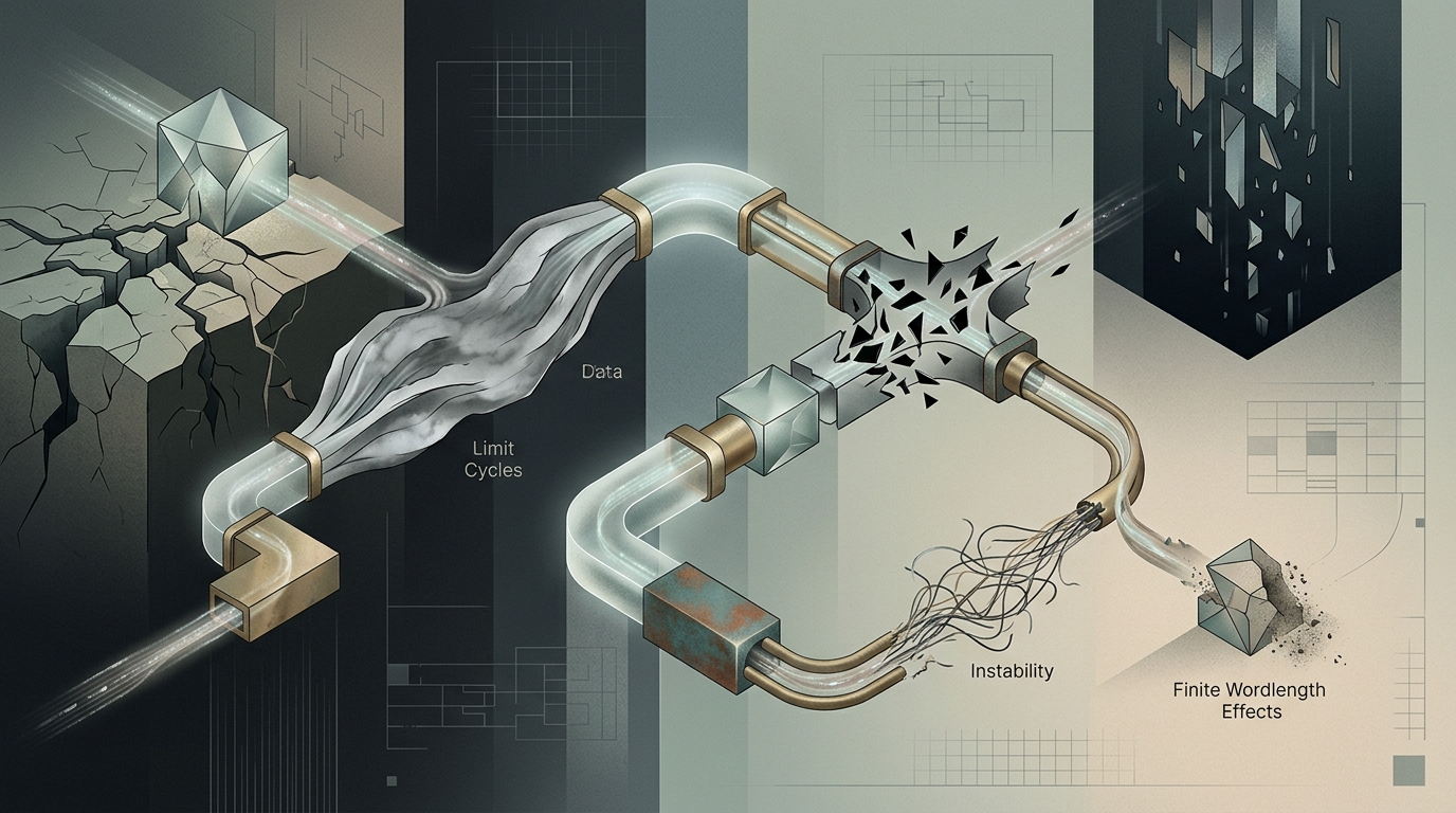
IIR filters don't fail like hardware. They fail like math. The three patterns I keep seeing are coefficient quantization drift, limit cycles, and accumulator overflow, and all three trace back to the same root: the design was verified in floating-point and deployed in fixed-point.
Quantization drift is the sneakiest. Your poles sat comfortably inside the unit circle in the design tool. Then the coefficients got rounded to 16-bit fixed-point, and a pole at 0.998 became 1.001. The filter passed every bench test with small signals, then slowly diverged in production. High-order direct-form implementations amplify this sensitivity, which is exactly why the cascade of second-order sections exists: each biquad's poles quantize independently, keeping errors local instead of compounding.
Limit cycles are the zombie oscillations. With zero input, a properly dead filter should decay to silence. A fixed-point IIR can instead settle into a small persistent oscillation sustained entirely by rounding in the feedback path. In audio, that's a faint idle tone that only appears in quiet passages. The fixes are standard: more accumulator headroom, error feedback, or dithering the quantizer.
Overflow is the loud one. Intermediate values inside an IIR stage can exceed the input range even when input and output are both in range. Without saturation arithmetic, a two's complement wraparound turns a near-full-scale value into a full-scale value of opposite sign, which the feedback path then recirculates. That's not a click. That's a screech. Saturating accumulators and headroom scaling between sections are non-negotiable in fixed-point IIR work.
Every one of these is invisible in a floating-point simulation. Verify on the target arithmetic, not just the target algorithm. The FAQ below covers the decisions that come up most.
Frequently Asked Questions
When should I pick FIR over IIR? When phase linearity or guaranteed stability is worth paying for in latency and MACs: measurement systems, audio crossovers where phase matters, data communications. Pick IIR when efficiency and low latency win: EQ, control loops, anti-aliasing, live monitoring. Lyons' rule of thumb holds up: FIR when phase matters, IIR when it doesn't and cycles are scarce.
Why does everyone implement IIR filters as biquad cascades? Because high-order direct-form structures are numerically fragile. Splitting an eighth-order filter into four second-order sections keeps each section's coefficient quantization error and internal gain local, so the whole chain stays stable on fixed-point hardware. It costs a little more bookkeeping and buys a lot of predictability.
How much latency does an IIR filter add compared to FIR? An IIR's delay is typically a few samples and varies with frequency, versus a linear-phase FIR's fixed (N-1)/2 samples. The AES figure cited above puts a 128-tap FIR at about 1.3 ms at 48 kHz. An IIR doing a comparable magnitude response runs far below that, which is why live audio paths lean IIR.
What does "poles outside the unit circle" actually mean for my system? It means the feedback gain exceeds unity at some frequency, so instead of decaying, energy grows every pass through the loop. In practice you hear oscillation or watch the output rail. Check pole radii after coefficient quantization, not before. The design tool's poles are not the poles your hardware runs.